Hey, I am Neil

A data enthusiast with more than 4 Years of I.T. experience in statistical analysis, IT Service Management and QA automation. This Portfolio presents different Projects which I undertook during my Post graduation in Data Analyst.

Contact Me @

Email Address : neilsahay996@gmail.com

Project 1:Factors-affecting-Covid-19

• The project aims to generalize the effects of Novel coronavirus across different counties in United States Of America and moreover discuss various different factors affecting the same. We have taken into account multiple age factors which are getting affected due to the virus and moreover takes into account different condition factors. The project looks to find distinct and diverse factors in various age groups, i.e. how they are impacting Covid deaths and cases across various regions in United States. The domain of the datasets is related to health care as discussed above the project aims to identify the impact of Covid. The datasets have been selected to take into account all these factors so as to combine diverse factors to get a generalized sense from the available data. The data is obtained mainly from Centre for Disease Control and Prevention which is Federal organization collecting data on daily or random basis as per their availability, moreover as per their description states and local authorities reports the cases regularly to keep the data up to date.

Data Pre-processing

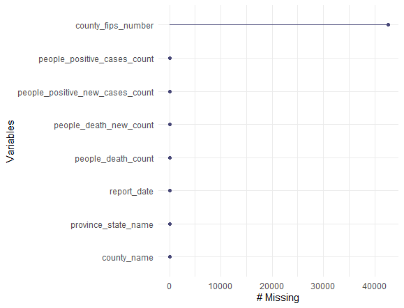
• To analyze the Null values in a more quantitative and generalized manner, we use different packages such as naniar which can give the number of missing values by plotting it and thus giving us a visualization to get more insights,fig. shows the implementation of naniar package

  

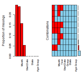
• VIM (Visualization and Imputation of Missing Values) package helps to visualize the missing data in a deep way and thus can help to apply specific mechanisms which can be helpful in analyzing the missing values and deciding whether to impute/replace or remove it, while Fig Shows the implementation of VIM package.

  

• Regression Techniques Implemented:

1. XGBoost
2. Random Forest
3. Multiple Linear Regression
4. Decision Tree

• Classification Models Implemented:

1. KNN(K-Nearest Neighbor)
2. SVC(Support Vector Classification)

Project 2:Time series analysis

Analysis of different time series models on OverseasTrips and NewHouseRegistrations in Ireland. Th project makes use of different time series analysis models such as ARIMA, Naive, Simple Exponential Model, etc. Below is a short description of data set and how it is analyzed for a time series model.

OverseasTrips Dataset

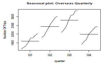
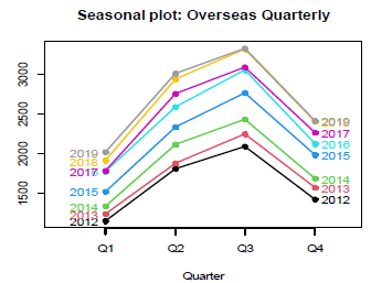
• The Overseas Trips dataset is obtained from Central Statistics Office in Ireland and is a quarterly time series data indicating travel by non-residents to Ireland from Q1. 2012 to Q4, 2019. In this section, we will analyze the raw time series of the dataset which is also the required step in every time series modeling process. As the raw time series helps to identify the Trends or Seasonality patterns within the data, which we can take into consideration during the execution of the models.

• Firstly the dataset extracted, is converted to a time series model using the function ts(), where the start and end is given along with the frequency and as this is a quarterly dataset, we given the frequency as 4. Moving on we plot the data using the function plot for which the output obtained is shown below in Fig. 1. ,which shows that there is increasing trend in the data as we move along from 2012 to 2020 moreover the plot also indicates the presence of seasonality which although remains constant for most time but also show spikes as the years progresses.:

MODEL BUILDUP PHASE

• In the model construction phase, we apply 3 different types of time series model to access the overseas trips dataset using various strategies such as smoothing models which we made use on this dataset. The different time series methods opted are Simple Exponential Smoothing, Holt’s model and lastly Holt winter seasonal method. The advantage of using exponential is that weights are given to observations with respect to recent and past data, with past data getting lower weights and new data getting higher weights.

1. Simple Exponential Smoothing

Step 1: Analysis of Raw Data and creating train and test:

The first step involves converting the raw data to time series data and as we have a quarterly time series data, we assign the frequency as 4 along with start and end parameters to convert the raw data to quarterly time series data. Then the data is extracted for the first 2 columns and then using the window (time series object, start, end) command in R, we subset the data into training and test sub-sets.

Step 2: Applying the model using alpha parameters best suited for SES:

SES gives best results by using the smoothing parameter i.e. alpha between the range 0.1 and 0.2, thus we apply the first initial model with alpha as 0.2 and number of forecasts i.e. ‘h’ as 3, on the train time series data. On plotting the modelled data using the function autoplot(), as shown in Fig. 5.,it is observed that we get a flat line showing that present trend is not captured properly, thus we need to remove the trend and seasonality from the data to make it stationary.

Step 3: Removing Trend and Seasonality from data:

To remove trend and seasonality from the time series data, differencing is used which make the non-stationary data with trend and seasonality as stationary data without trends and seasonality. As there is no reasonable variance observed therefore Logarithmic transformation is not used. To get the number of differencing required ndiffs(time series object) is used which gives the output as 1 Therefore we make use of command diff() command, to make the train and test data stationary.

Step 4: Detecting the optimal values for alpha: To get the optimal value of the smoothing parameter to achieve the minimum RMSE is an essential task in the model buildup process. Therefore to get the optimal value of the alpha parameter, we implemented a function which creates a sequence from 0.01 to 0.99, with an increment by 0.1 and calculating the RMSE on each value consequently.

1. Holt’s Exponential Smoothing Model Buildup

Step 1: Analysis and Creating train and test: As the process to convert the raw data to a quarterly time series data, is already achieved in the Simple Exponential Smoothing phase. Thus we move ahead with extracting data for the first 2 columns from the time series dataframe to a spate data frame and then using the window (time series object).

Step 2: Applying the model to get optimal beta values: Holt model is applied by using the function holt() passing the time series object along with alpha and beta parameters. For the initial model we don’t give any beta value as holt will assign a beta value which after doing the summary of the applied model we get the optimal value of beta as 0.0001, on which we can perform tuning by creating a sequence function which will increment till 0.5 and fitting each model with that specific beta value and obtaining the resulting RMSE, with the goal to achieve minimum RMSE, which comes out to be 0.0341 with RMSE as 547.

Step3: Applying the Holt’s model with appropriate beta values: The optimal gamma value obtained is 0.0341 with minimum RMSE, thus applying minimum beta value obtained in the model with number of forecasting periods as 3, gives an AIC of 375.

1. Holt’s Winter Exponential Smoothing Model Buildup

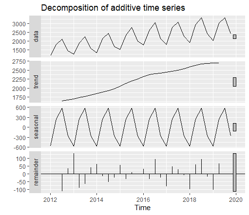
Step 1: Decomposition of different time series moreover analyzing the model parameters required: On converting the data to a time series data, we can decompose the time series into seasonal and trend obtained by making use of decompose() method and passing the time series object which disintegrates the model to seasonal ,trend thus indicating the parameters that should be passed in model attribute as shown in Fig. 15., indicating it as an additive time series mode for trend parameter while the seasonal variations observed indicate a Multiplicative time series approach, thus giving the final models as (M,Ad,M).

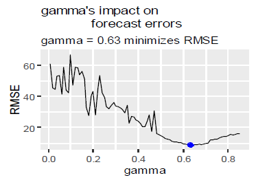
Step 2: Detecting optimal gamma values: The initial model applied gave the value of gamma as 0.0001.To detect the optimal gamma value, we again make use of the sequence function which increments till 0.85 and checks the RMSE obtained at each gamma value so as to obtain the minimum gamma showing the minimum RMSE. Thus the minimum gamma value is 0.63 for which minimum RMSE is obtained 8.77.

SUMMARIZING TO IDENTIFY OPTIMAL MODEL

On Overseas trips we applied three different time series models, starting with Simple Exponential Smoothing, followed by Holt’s Smoothing and finally Holt’s winter smoothing model. All the three models are thoroughly using loop execution to ensure we get the smoothing parameters which show the minimum RMSE obtained. Therefore after executing 3 different exponential smoothing models, we need to identify which time series model performed well on our data, thus we will run the below tests to evaluate the same:

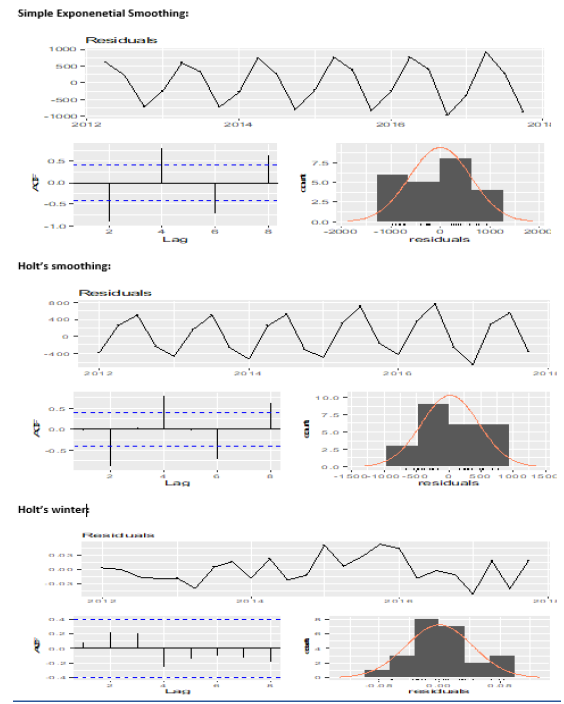
1.) Checking Residuals: Checking the residuals can be achieved with the help of R command checkresiduals$model. As observed from Fig.19. , it is evident that only Holt’s winter model has ACF plot in which no autocorrelation is observed as no spike is above the dotted line, while on the other hand in Simple seasoning model and Holt’s model ,the ACF plot shows high auto-correlation as the spikes are above the dotted lines.

2.) Validating using AIC (Akaike Information Criteria): The AIC obtained from all the three different exponential smoothing models is as follows:

a. Simple Seasonal Exponential Model AIC: 370.7959 b. Holt’s Exponential Model AIC: 375.8386 c. Holt’s winter model AIC: 283.4927

Therefore from the AIC values obtained from the summary of different models, we can conclude that the model with least AIC observed i.e. 283 in Holt’s winter model is the best fit model on the data.

New House Registration Dataset

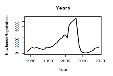
• TThe dataset contains annual time series data of new house registrations of the past 42 years i.e. from 1978 to 2019. We will implement 3 different times series models i.e. ARIMA(Auto Regression Integrated Moving Average), mean model and naïve model. Before starting to implement the above models, we will plot the raw time series data to find out and analyze any trends or seasonality. Below graph in Fig. 20 shows increasing trend from 1978 to around 2005 or 2006 and then it starts decreasing and again seems to be increasing. Thus we can conclude from the analysis that we have trend in our raw time series data.

Before starting to implement the above models, we will plot the raw time series data to find out and analyze any trends or seasonality. Below graph in Fig. 20 shows increasing trend from 1978 to around 2005 or 2006 and then it starts decreasing and again seems to be increasing. Thus we can conclude from the analysis that we have trend in our raw time series data.

ARIMA Modelling:

In the process of execution of ARIMA modelling technique[3], it is important to remove trend or seasonality from the time series data, and as in analysis f raw time series data, only trend pattern is detected we will apply aim to remove trend pattern. Below steps will explain the same:

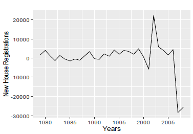
Step 1: Analyzing the data for patterns: The first step is to remove any trend or seasonality pattern from the time series dataset, as in ARIMA model any trend or seasonal pattern is not preferred. As the data had trend present, we use ndiffs() command to get the number of differencing required to make the data stationary.

Step 2: Implementing Augmented Dickey Fuller test: To ensure that the data is stationary, we perform Augmented Dickey Fuller test, which on analyzing should give the p-value less than 0.5 thus confirming the null hypothesis, that the data is stationary.

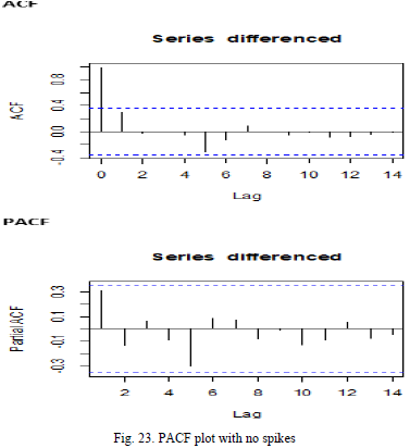
Step 3: Examining the ACF and PACF Plots to identify models and values of p and q: ACF(Autocorrelation function) and PACF(Partial autocorrelation function) helps to identify the type of ARIMA model which should be implemented. The ACF plot shows a single spike and then slowly decay as shown in Fig.23. , while the PACF plot does not show any spikes as shown in Fig. 23. Therefore we can confirm that this a Moving average model i.e. MA(1) model with p value observed as 0 and q value observed as 1.

Step 4: Fitting the ARIMA model with values of p, d and q and also using auto ARIMA: The values to be put in our model are 0 for p, differencing is 1 and q as 1 which concludes to ARIMA(0,1,1). Therefore the equation to fir the model is arima(object,order=c(0,1,1)). Thus we get the value of ma1 as 0.3736 with AIC (Akaike Information Criteria) as 627.86. Now we make use of auto.arima(time series object, stepwise=FALSE) function to get the optimal model by automating the arima process, here the stepwise is given as FALSE so that we can detect all the possible combinations. Thus the model obtained from auto.arima came to be ARIMA(1,1,0), thus contradicting the fact that the model is MA(1) model and not an AR(1) model.

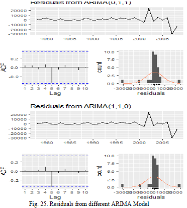
Step 5: Checking the residuals to ensure white noise observed: On plotting the residuals on QQ plot as shown in Fig. 24., we observe that for both the models i.e. ARIMA(0,1,1) and ARIMA(1,1,0) ,the residuals are normally distributed and moreover performing the checkresiduals(model$residual) test which is an automated version of Ljung Box test as shown in Fig. 25., we do not get the significant p-values for both the ARIMA models but the better value is obtained for ARIMA(1,1,0) model and thus we can conclude that the residuals are independently distributed thus showing the models have white noise.

Other Modelling Techniques are described in the respository

• Please click on the link of Project to visit the repository.

SUMMARIZING TO IDENTIFY OPTIMAL MODEL

As both the naïve method and simple moving average belongs to the same class, we will compare these 2 models with each other first and then the resulting would be compared with ARIMA model. Comparing Naïve and Simple Moving Average gives the standard deviation of the simple moving average as 8667.4, while in Naïve model gives a standard deviation 8521.7195, thus showing that Naïve model performed better than Simple Moving Average.

Comparing the ARIMA model with Naïve model, the former gives an RMSE of 8521.719 while for ARIMA gives an RMSE of 7736.531, while for MAE Naïve model gives 4681 while ARIMA again gives a lower value of 3863.819, thus showing that of all the three models observed ARIMA has scored better

Project 3:Business-Intelligence-and-Business-Analytics

This was a group project in which I had a team of 2 members and our task was that we have been hired from Olist firm with intend to increase Sales and Profit Margins. We have to perform analysis on the current system, and we have to come up with the approach to implement full business intelligence suite which will give better Insights on the Customer and Sales. Olist is Start-up in Brazil in E commerce industry. The Main objective is to analyse the Gaps in the current System and give the low-cost scalable Business intelligence system.

Business Background, Marketplace Information and Operations

• Olist Store is a very large departmental store in Brazil and it connects various small stores across the country on a single platform without any issues. As many stores are in the rural areas which though having products are not able to sell across the country due to logistic issues and most important factor to outreach the large consumer base. Through integration with Olist marketplace, such small and medium level stores are given the opportunity to expand their consumer base across regions which were earlier not part of their manifesto.
• The marketplace under which Olist operates comes under E-commerce, which has seen a rapid increase in the consumer base. In Latin –America, Brazil has a strong place in the e-commerce market with a market share closing to around 43%. As many rural areas in Brazil are able to access things outside their regions via mobile phones, thus attracting a large consumer base, and with a market share approaching 50 percent share in the entire Latin America, Brazil as a country cannot be ignored as a prospective marketplace considering the large population and ownership of cashless payment facilities mainly through credit cards. Moreover the increasing mobile commerce across the country with a significant percentage of approximately 40 percent just next to United States of America, makes Brazil as the forerunner in the prospect of E-commerce business.

Tableau Powered Dashboards

As the scope of E-commerce is increasing day by day across different regions, we as Olist try to help our consumers which in this case are our sellers to help increase their business growth so that more and more sellers from different regions can be part of Olist eco-system which provides end to end demand and forecast handling in dealing with the customers. We have connected our Tableau directly with the database hosted on Azure SQL Server. The below figure shows Tableau direct connection with SQL Server, with database selected as BIBA_PROJECT and tables designated below the same.

Story Line for our Payments Segregation Dashboard

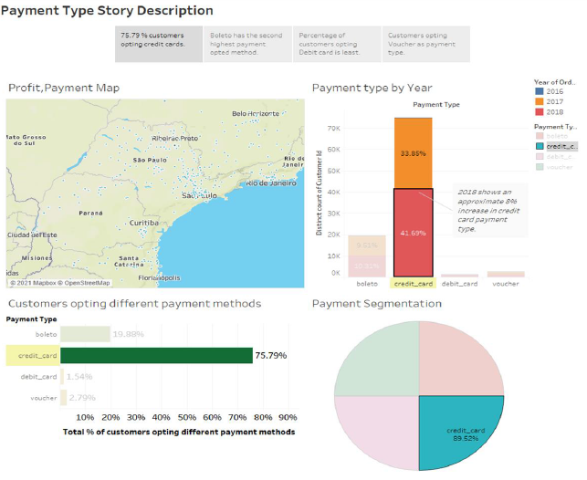
Credit card as a payment type

Credit card is the most common type of payment method prevalent across the entire globe, where the consumer even if don’t have sufficient money in their accounts can make the payments. Therefore on selecting the credit card as payment type in highlighter, Tableau is able to highlight the key parts in the entire dashboard. Below are the core modules and insights shown by our interactive dashboard.

1. Credit card accounts for approx… 90 percent of Payment segmentation, showing that many distinct payments are made through credit cards.
2. Approximately 78 % consumers opted credit card as the mode of payment, this gives us an interesting insight which can be used by our sellers to promote their products.

3. In 2016 credit card payments accounted merely 0.25 %, but increased in 2017 by 30%, owing up to 34 % and in 2018 accounted for 45%.

   

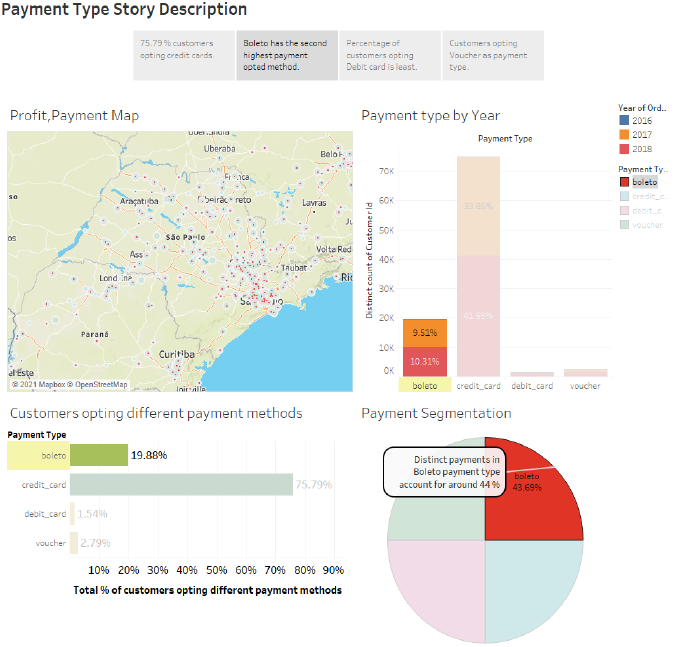
Opting Boleto as a payment type

Boleto is a type of payment system in Brazil which is regulated by FEBRABAN, which is short for Brazilian Federation of Banks. Boleto’s can be used across different ATM machines, Outlets, Online Transactions and superstores till the expiration date. Our dashboard below highlights some of the important aspects mentioned below:

1. Boleto as payment type accounts for approximately 20 percent as preferred payment type, second most after credit card usage.
2. Around 43.69 % distinct payments came through boleto payment type, again second most after credit card.

3. Payment type by year shows increasing trend ion usage of boleto as payment type, with stats as 0.06 % boleto usage in 2016, followed by approx… 10% in 2017 and finally 10.31% in 2018.

   

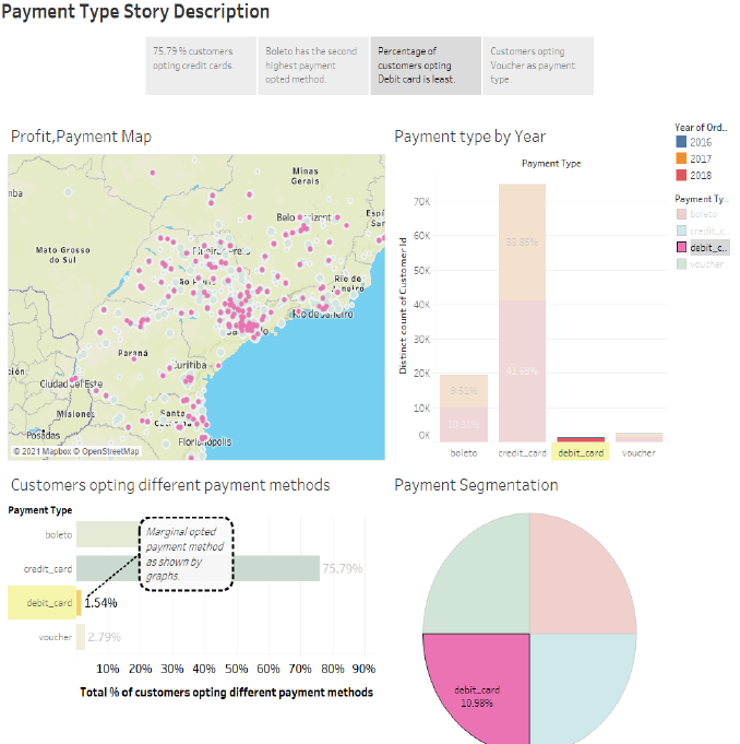
Opting Debit Card as a payment type

Debit card is the least opted payment method opted by the consumers while buying products through Olist. The below observations describes the insights retrieved from the dashboards.

1. Marginally 2% of consumers opted for Debit card as their payment method as can be concluded from the dashboard.

2. While in 2016, debit card did not accounted for any transactions through Online payments via Olist , the figure marginally increased in the following year coming to 1.11%.

   

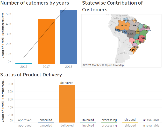
Customers Insights

The next Dashboard Gives information regarding Customer Insights.The First Bar Graph represents no. of customers by years like we can see in year 2016 we have less customers but there was a huge surge in the year 2017 which got increased from to 44,000 and then in year 2018 we again see huge margin increment in the no of customers of about 15000 customers.So already we can see lot of people start using E commerce websites for there buisness.We have also plotted the Demographic map which shows state wise Contribution of Customers and this Map tell us that Sao Paulo has highest no of customers in the year 2017 with count of 17.52 K customers, which finally got increased to 23.74 k customers in the year of 2018.As the Dashbiard is interactive we can see no of delivred product is also changing yearly.Also we can see delivered item also got increased which was natural as the no of cutomers got increased. We have also plotted Regression line in witn adjusted R Square 87 percent and the p value of 0.27 which is less then 0.5 means we are nearly correct in our Analysis.

Project 4:Analyzing Covid-19 Deaths in Patients with Different Conditions among Various Counties in the United States of America

As a group project comprising of 2 team memebers, this repository presents the work done by me, moreover there are 2 Jupyter Notebooks uploaded, and it contains analysis performed on Coivd-19 using Pandas dataframes, numpy, regression techniques and No-SQL databases design. The datasets has been acquired from CDC though Socrata API, and retreived in python by using limit parameter. Please clcik on the highlighted link to move to the particular repository and get more insights.)

Below is the abstract, detailing about the problem faced and how it will be tackeled thorugh this research.

• Since the spread of Covid-19 virus which has impacted the whole world, dislodging some of the world’s biggest economies to the bottom with no exception of the United States of America, the death rates across America spiked at a tremendous rate therefore causing tremendous loss of life. Thus such an impact around the world has been a motivation for the research, so as to evaluate the covid-19 mortality among various counties with patients suffering under various conditions such as some patients have septic, influenza and many other moreover finding the probable cases so as to predict the mortality rates of the region, which can help the counties to take measures to avoid such an outcome.

• The study aims to analyze various patients’ under different categories of their respective health status. The research in the topic helped to generalize the data in a more efficient manner so as to analyze the Covid deaths across various counties moreover exploring new insights in the hidden data such as number of probable deaths, new cases, updated probable deaths, identifying different age groups and their corresponding symptoms.

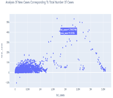
• Scatter plot:

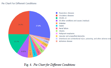
• Pie chart showing patients with different conditions affected by covi-19

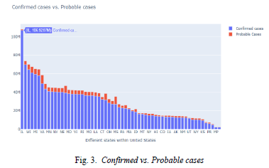
• Bar chart showing Probable vs. Confirmed cases